
Buy a license here (or from Help->Licensing in FlowCompute to have your MachineID automatically filled in).
How it works
I came up with a new way to do math using two powerful tools: flow charts and reusable sets of equations.
The workflow goes something like:
- Create a project, which can contain multiple “Flows”.
- Create a bunch of nodes that are either A) input values, B) outputs, C) math operations, or D) equations.
- Link them together by their input and output sockets, creating the flow chart.
- Read the solution from the output nodes, or plot the result graphically.
- Optionally: Export results to Excel, a CSV file, or Blender.
- Optionally: Print the complete set of math calculations that were done to arrive at the result (hard proof that the result is correct!)
All of the simple math is handled by math nodes. All of the complex math is handled by Equation Definition files, which are designed once per equation and then can be reused and shared in the future.
It also understands units and unit conversions. For example, it is perfectly valid to multiply pounds (force) * meters (length) and get the result in oz-in (torque). The conversion factors and relationships are handled internally which simplifies the math greatly from the user’s point of view. Units are fully customizable if you need units that are not built in.
You can also change inputs to be variables and plot the result of any output, allowing you to effectively analyze and graph complex relationships without worrying about the details of the math behind it.
Finally, it provides a list of all of the mathematical calculations performed and equations used.
Example: 2 car collision
Let’s take a look at a flow that does a conversation of momentum analysis. The scenario is: a 2000 Ford Explorer rear-ends a 1995 Honda Civic. The Civic was stopped at a stop light. They both exit the collision at the same speed (stuck together). The Explorer was travelling at 50MPH at impact. What was the delta-V for the Civic?
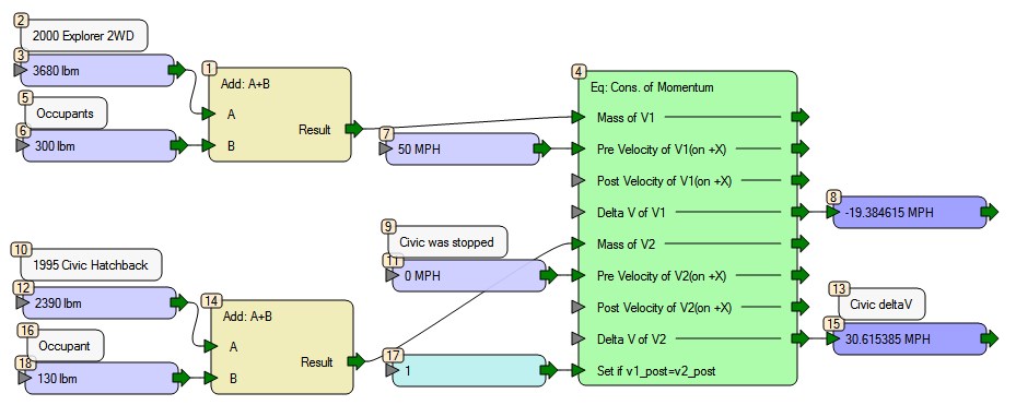
So the answer is 30.6MPH, and we didn’t have to do any math to arrive at that. The math is readily available, however, if we need to prove the work to someone else. Here’s a (very short) snippet of the output:
For Node 1:
Math Operation: Add: A+B

Given:
A = 3680 lbm
B = 300 lbm

Solved: Result = 3980 lbm


---------------------------------------------------

For Node 4:
Using equation system: Cons. of Momentum

Given:
v1postisv2post_flag = 1
m1 = 3980 lbm
v1_pre = 50 MPH
m2 = 2520 lbm
v2_pre = 0 MPH

Solved: v1_post = 30.615385 MPH
Using equation/code: v1_post=(m1*v1_pre+m2*v2_pre)/(m1+m2);
Example: Graphing
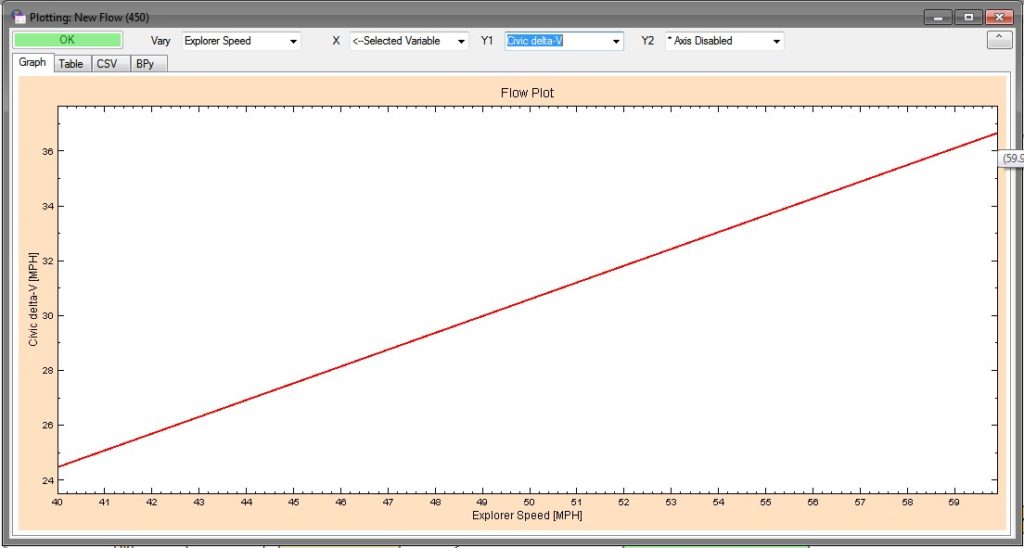
Now, what if we didn’t know the Explorer’s speed for certain and we want to find out what happens over a range of values? It’s easy enough to change the input speed node and read the output, but we can also graph it by switching the Explorer’s speed input to a Variable and linking the Civic’s delta-V output to a Plotter.
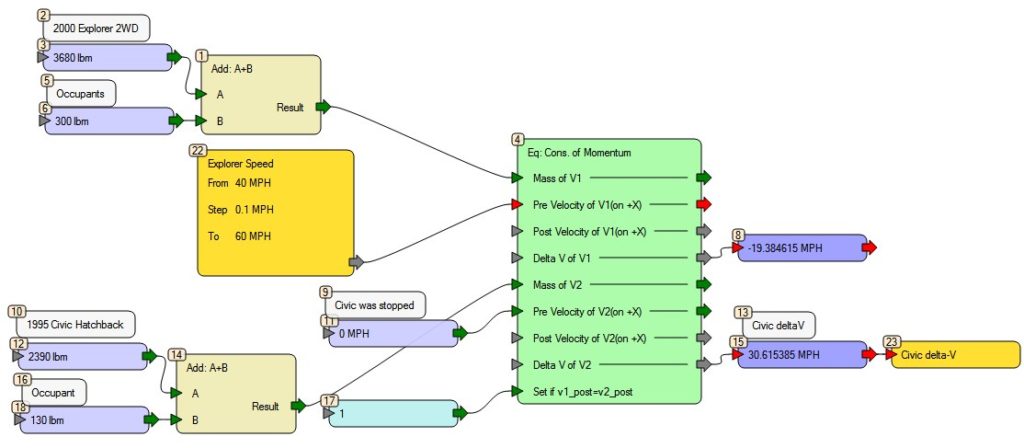
Having a variable and a plotter (or two!) allows you to view the result in graphical and tabular format.
That’s all for now. More examples to come!